Authors: Tanveer Mittal & Andrew Shen
Mentor: Arun Kumar
The following is an abbreviated technical report for our Senior Data Science Capstone at UC San Diego. This project is an extension of Project SortingHat of the ADALab at UCSD and was conducted under the mentorship of Professor Arun Kumar.
Artifacts:
- Model Training and Experiment Code
- Provides all our code for experimentation and model training
- PyTorch Hub Release of Pretrained Models
- Allows anyone to load our models in a single line of code using the PyTorch Hub API!
- Tech Report
- Provides detailed methodology and results of our experiments
Resources:
- ML Data Prep Zoo
- Provides benchmark data and pretrained models for Feature Type Inference
- Project Sortinghat
- Home page of Project SortingHat which provides their previous work on this subject
Introduction
Automated Machine Learning(AutoML) has grown in popularity recently as it has enabled scalable ML for the masses. Currently the machine learning pipeline has a lot of manual steps such as data preprocessing and model building. AutoML platforms and soft- ware aim to automate the entire ML pipeline. Many such platforms already exist such as Amazon Sagemaker, Google Cloud AutoML, Salesforce Einstein and more. As a result the different steps involved in the AutoML pipeline are heavily researched in academia as well.
The first step AutoML software must take after loading in a dataset is to identify the feature types (ie numeric, categorical, datetime, …) of individual columns in the input data. This feature type inference information allows the software to understand the data and preprocess it to allow machine learning algorithms to run on it. Feature type inference is still being done manually by data scientists which in most cases becomes impractical as dataset can have hundreds or more features that require labeling. Previous tools have also implemented automated Feature Type Inference using rules-based prediction.
Project Sortinghat of the ADA lab at UCSD frames this task of Feature Type Inference as a machine learning multiclass classification problem. Machine learning models defined in the original SortingHat feature type inference paper use 3 sets of features as input.
- The name of the given column
- 5 sample values from the data to be used as base features
- Descriptive numeric statistics computed from the entire given column (Listed in Table 1)
The textual features such as the column name and the 5 sample values are easy to access, however the descriptive statistics models rely on a full iteration through every row and value in the data which make preprocessing less scalable as the dataset size grows. Our goal is to investigate 2 questions about feature type inference:
- Can we take the Random Forest Model from Project Sortinghat and investigate how adjusting the number of base feature sample values or taking a subsection of the data for descriptive statistic calculation affects the model?
- Can we experiment with and apply deep learning transformer models to feature type inference to improve accuracy and scalability further?
Previous Work
Project SortingHat produced the ML Data Prep Zoo which is a collection of publicly available datasets. The zoo also includes all the precomputed features defined above as labeled benchmark data for feature type inference. This data plays a role in this space similiar to ImageNet in computer vision allowing the benchmarking of existing tools on this task. For our investigation, we have used the original data from the ML Data Prep Zoo; both the raw csv’s of data as well as the benchmark labeled data to train and test our models with.
The SortingHat paper also proposed and used a set of 9 class labels; We continue to use these 9 class labels for our models as labeled in the benchmark dataset. The experiments observed in the original SortingHat paper produced models that outperform the accuracy of existing tools such as AWS’s AutoGluon, Google’s Tensorflow Data Validation, the Pandas python library, and more. The single best model produced by this paper was a random forest model that uses the column name and descriptive statistics that yielded an Accuracy of 0.9265.
| Descriptive Statistics |
|---|
| % of nans |
| % of unique values |
| Mean and std of column values, word count, stopwordcount, count, char count, whitespace count, and delimiter count |
| Min and max value of the column |
| Regular expression check for the presence of url, email,sequence of delimiters, and list on sample values |
| Pandas timestamp check on sample values |
| Numeric | 0.97 |
| Categorical | 0.97 |
| Datetime | 0.99 |
| Sentence | 0.99 |
| URL | 1.00 |
| Embedded Number | 0.99 |
| List | 1.00 |
| Non-Generalizable | 0.98 |
| Context Specific | 0.96 |
Methods
Random Forest Investigation
As mentioned above, Project SortingHat’s best performing model was a Random Forest that achieved an accuracy of 0.9265 overall and class wise accuracy shown in Table 2. This was generated using 5 sample values from the data column as base features and using the Table 1 set of descriptive statistics calculated using the entire data column. To further investigate the performance of this random forest model and to answer the first question on feature type inference we will be adjusting both the number of sample values used as base features and the subset of data used to calculate the descriptive statistics
To investigate ways of improving model runtime and accuracy, we will first experiment with adjusting the number of sample values used as base features. The original Random Forest Model was trained using 5 sample values, but for our experiment we tested using 1,2,3,4,5, and 10 sample values as base features. As expected, when using 5 sample values in the base feature set, our model is exactly the same as the original SortingHat Random Forest and produces the same accuracy values.
| Number of Sample Values in the Base Features | 1 | 2 | 3 | 4 | 5 | 10 |
| Feature Type | ||||||
| numeric | 0.97 | 0.97 | 0.97 | 0.97 | 0.97 | 0.97 |
| categorical | 0.97 | 0.97 | 0.97 | 0.97 | 0.97 | 0.97 |
| datetime | 1.00 | 1.00 | 1.00 | 1.00 | 1.00 | 1.00 |
| sentence | 0.99 | 0.99 | 0.99 | 0.99 | 0.99 | 0.99 |
| url | 1.00 | 1.00 | 1.00 | 1.00 | 1.00 | 1.00 |
| embedded-number | 0.99 | 0.99 | 0.99 | 0.99 | 0.99 | 0.99 |
| list | 0.99 | 0.99 | 0.99 | 0.99 | 0.99 | 0.99 |
| not-generalizable | 0.98 | 0.98 | 0.98 | 0.98 | 0.98 | 0.98 |
| context-specific | 0.96 | 0.96 | 0.96 | 0.96 | 0.96 | 0.96 |
What is discovered in Table 3 is that the Random Forest accuracy is not noticable affected by either an increase or decrease in the number of sample values used in the base feature set. Between using only 1 random sample from the data column as a base feature to using 10 random samples as base feature that accuracy did not change more than 1%.
Additionally, increasing the number of sample values used as base features did not have as much of an impact on the model runtime as expected. We measured the time it took to train and test the model across all 1 though 5 and 10 base feature sample values over 3 iterations. Between including only 1 sample value as a base feature compared to including 10 samples as a base feature, there was a less than 1% time increase between 1 and 10 sample models
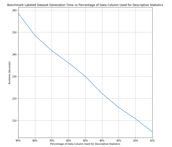
A time consuming step of the feature type inference process is the calculation of descriptive statistics. As referenced in Table 1, all the descriptive statistics require a complete iteration to calculate the values used in the ML model. Our experiment involves taking subsets of data, sampled randomly without replacement, from the entire data column at 10% intervals (ie 90%, 80%, …). For example if a data column has 1,000 values and we are taking a 50% subset, we would sample 500 values to use in the calculation of our descriptive statistics. This will reduce the number of value that we will have to iterate over, increasing the calculation speed of the descriptive statistics. The downside is the loss of information and inaccuracy in the descriptive statistics caused by now using all available values in the data column. In this experiment we are keeping the 5 sample values in the base feature set as we have seen they do not have much of an effect on either accuracy or runtime.
| Percentage of Data used to calculate descriptive statistics | 90% | 80% | 70% | 60% | 50% | 40% | 30% | 20% | 10% |
| Overall Model Accuracy | 0.902 | 0.900 | 0.900 | 0.893 | 0.894 | 0.899 | 0.891 | 0.892 | 0.886 |
As seen in Table 4, there is a constant decrease in model accuracy as we lower the proportion of the data we are using to calculate our descriptive statistics with. For more detailed metrics, Table 5 shows the class wise metrics across the different proportions we are taking from the data column. From Table 5 we can see that Categorical sees the largest decrease in accuracy as we take a smaller proportion of the entire data set for descriptive statistic calculation, with notgeneralizable and context-specific feature types also affected. This makes sense as these feature types require looking at much more of the data compared to feature types such as URL or datetime.
Although accuracy increases as we use more of the data column for descriptive statistic calculation, so does the runtime. Figure 1 displays the change in runtime of the descriptive statistic calculation as used for the benchmark labeled data test set. Though the training set has more columns and features to calculate, the test and train runtimes follow the same linear pattern as we adjust the proportion of data we subset. In the calculation of the benchmark labeled data, the descriptive statistic runtime is only affected by the number of values in the data column that we are inferring the feature of. As we adjust what percentage of the data column we subset for our statistic calculations, there is a linear decrease in runtime. Using Table 4, Table 5, and Figure 1, we can adjust how to best balance optimizing runtime through only selecting a percentage of the entire data column for the descriptive statistics and our accuracy requirements.
| Proportion of Data Column Used to Calculate Descriptive Statistics | 10% | 20% | 30% | 40% | 50% | 60% | 70% | 80% | 90% | |
| Feature Type | Metric | |||||||||
| numeric | accuracy | 0.97 | 0.97 | 0.97 | 0.97 | 0.96 | 0.96 | 0.97 | 0.97 | 0.97 |
| precision | 0.93 | 0.93 | 0.93 | 0.93 | 0.92 | 0.92 | 0.93 | 0.93 | 0.93 | |
| recall | 0.98 | 0.98 | 0.98 | 0.99 | 0.98 | 0.98 | 0.98 | 0.98 | 0.98 | |
| f1-score | 0.95 | 0.96 | 0.95 | 0.96 | 0.95 | 0.95 | 0.95 | 0.95 | 0.96 | |
| categorical | accuracy | 0.93 | 0.94 | 0.94 | 0.94 | 0.94 | 0.94 | 0.94 | 0.94 | 0.95 |
| precision | 0.83 | 0.84 | 0.84 | 0.87 | 0.86 | 0.85 | 0.86 | 0.86 | 0.86 | |
| recall | 0.89 | 0.91 | 0.91 | 0.90 | 0.90 | 0.90 | 0.90 | 0.91 | 0.91 | |
| f1-score | 0.86 | 0.87 | 0.87 | 0.88 | 0.88 | 0.88 | 0.88 | 0.88 | 0.89 | |
| datetime | accuracy | 1.00 | 0.99 | 1.00 | 1.00 | 1.00 | 1.00 | 1.00 | 1.00 | 1.00 |
| precision | 0.98 | 0.96 | 0.99 | 0.97 | 0.99 | 0.99 | 0.97 | 0.98 | 0.98 | |
| recall | 0.98 | 0.96 | 0.96 | 0.98 | 0.97 | 0.97 | 0.96 | 0.96 | 0.96 | |
| f1-score | 0.98 | 0.96 | 0.97 | 0.97 | 0.98 | 0.98 | 0.97 | 0.97 | 0.97 | |
| sentence | accuracy | 0.99 | 0.99 | 0.99 | 0.99 | 0.99 | 0.99 | 0.99 | 0.99 | 0.99 |
| precision | 0.89 | 0.87 | 0.87 | 0.88 | 0.87 | 0.88 | 0.90 | 0.89 | 0.91 | |
| recall | 0.86 | 0.82 | 0.82 | 0.86 | 0.87 | 0.87 | 0.88 | 0.88 | 0.87 | |
| f1-score | 0.88 | 0.85 | 0.85 | 0.87 | 0.87 | 0.87 | 0.89 | 0.88 | 0.89 | |
| url | accuracy | 1.00 | 1.00 | 1.00 | 1.00 | 1.00 | 1.00 | 1.00 | 1.00 | 1.00 |
| precision | 1.00 | 0.97 | 1.00 | 1.00 | 1.00 | 1.00 | 1.00 | 1.00 | 1.00 | |
| recall | 0.81 | 0.91 | 0.97 | 0.91 | 0.94 | 0.94 | 0.94 | 0.94 | 0.94 | |
| f1-score | 0.90 | 0.94 | 0.98 | 0.95 | 0.97 | 0.97 | 0.97 | 0.97 | 0.97 | |
| embedded-number | accuracy | 0.99 | 0.99 | 0.99 | 0.99 | 0.99 | 0.99 | 0.99 | 0.99 | 0.99 |
| precision | 0.89 | 0.92 | 0.91 | 0.95 | 0.91 | 0.90 | 0.92 | 0.92 | 0.92 | |
| recall | 0.86 | 0.87 | 0.88 | 0.89 | 0.87 | 0.90 | 0.88 | 0.88 | 0.88 | |
| f1-score | 0.87 | 0.89 | 0.89 | 0.92 | 0.89 | 0.90 | 0.90 | 0.90 | 0.90 | |
| list | accuracy | 0.99 | 0.99 | 0.99 | 0.99 | 0.99 | 0.99 | 0.99 | 0.99 | 0.99 |
| precision | 0.83 | 1.00 | 1.00 | 0.83 | 0.80 | 0.80 | 0.86 | 0.80 | 1.00 | |
| recall | 0.28 | 0.21 | 0.21 | 0.26 | 0.21 | 0.21 | 0.32 | 0.21 | 0.32 | |
| f1-score | 0.42 | 0.35 | 0.35 | 0.40 | 0.33 | 0.33 | 0.46 | 0.33 | 0.48 | |
| not-generalizable | accuracy | 0.95 | 0.96 | 0.96 | 0.96 | 0.96 | 0.96 | 0.96 | 0.96 | 0.96 |
| precision | 0.81 | 0.84 | 0.84 | 0.85 | 0.85 | 0.84 | 0.86 | 0.86 | 0.86 | |
| recall | 0.75 | 0.79 | 0.78 | 0.81 | 0.80 | 0.77 | 0.80 | 0.80 | 0.79 | |
| f1-score | 0.78 | 0.81 | 0.81 | 0.83 | 0.83 | 0.81 | 0.83 | 0.83 | 0.82 | |
| context-specific | accuracy | 0.96 | 0.96 | 0.95 | 0.96 | 0.96 | 0.96 | 0.96 | 0.96 | 0.96 |
| precision | 0.83 | 0.85 | 0.82 | 0.85 | 0.84 | 0.83 | 0.86 | 0.84 | 0.84 | |
| recall | 0.70 | 0.69 | 0.67 | 0.68 | 0.68 | 0.69 | 0.71 | 0.72 | 0.72 | |
| f1-score | 0.76 | 0.76 | 0.74 | 0.75 | 0.75 | 0.76 | 0.78 | 0.78 | 0.78 |
Transformer Models
In the hopes of creating more accurate and scalable models, we applied deep learning transformer models to feature type inference. We are using transformers to generate contextualized embeddings for words present in the column name and sample values of a column. As transformers currently produce state of the art results on natural language processing tasks, we hypothesise transformer models will be able to perform well on feature type inference because of their ability to generate contexualized word embeddings. This means that embeddings will be encoded with relevant information from other words in the same sequence. We believe these models will be able to better leverage the column names and sample values in context to each other.
In this project we specifically experimented with the Bidirectional Encoding and Representation Transformer(BERT)\cite{bert} model pretrained by Google to generate embeddings.
To preprocess the column names and samples values we concatenated them and used separation([SEP]) tokens between them. These single strings are then tokenized using the HuggingFace transformers library. Our best model’s architecture can be seen in Figure 2. BERT receives the text and then outputs a sequence of embeddings of size 768.
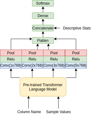
We then use a convolution neural network architecture to process BERT’s embeddings. This is inspired from a paper that uses BERT with a CNN for offensive speech classification\cite{bert_cnn}. In this original model, the sequence of embeddings is fed into 5 separate convolution layers that are processed with pooling and activation functions in parallel. The intuition behind this operation is that the different convolution filter dimensions can analyze different types of ngrams present in our data. Theoretically this model is able analyze individual words, bigrams, trigams, and more. The output of these operations are then concatenated and flattened. This convolution output is then concatenated with the descriptive statistics and fed into a softmax dense layer to output a classification.
Architecture Experiments
This architecture has a lot of hyperparemeters and architeture that can be changed so we decided to run a series of experiments to identify the best combination of convolution blocks and kernel size our CNN can use for this task. Our experiment results can be seen in our tables below. From these results we identified our best architecture to be one that uses 4 convolution blocks with filter dimensions of [1, 2, 3, 5] and a kernel size of 256 for each convolution layer.
| Convolution Filters | [1, 2, 3, 4, 5] | [2, 3, 4, 5] | [1, 3, 4, 5] | [1, 2, 4, 5] | [1, 2, 3, 5] | [1, 2, 3, 4] |
|---|---|---|---|---|---|---|
| Validation Accuracy | 0.931 | 0.924 | 0.924 | 0.926 | 0.928 | 0.930 |
| Testing Accuracy | 0.930 | 0.928 | 0.931 | 0.929 | 0.934 | 0.932 |
| Delta % Testing Accuracy | 0.00% | -0.15% | +0.15% | -0.05% | +0.35% | +0.25% |
| Kernel Size | 64 | 128 | 256 | 384 | 512 |
|---|---|---|---|---|---|
| Valid Accuracy | 0.923 | 0.929 | 0.931 | 0.929 | 0.930 |
| Test Accuracy | 0.928 | 0.930 | 0.934 | 0.930 | 0.933 |
Feature Experiments
To analyze the importance of different feature sets, we decided to run an ablation experiment for different combinations of feature sets these models are trained on. We could not run an experiment only using descriptive statistics as this would not use a transformer model in our architecture, so every other combination’s results are documented in Table 8.
We can observe in these results that BERT is better at analyzing the textual features than any of the models from the original SortingHat paper. The sample values are suggested here to be the single most important feature for our model. This supports our hypothesis by suggesting that BERT is effectively leveraging sample values with the context of each other. Our best model from this experiment is still the one using all of our features, however unlike the results from original SortingHat paper, the accuracy improvement of using the descriptive statistics is very small. In fact our model that only uses column names and sample values still outperforms the previous best random forest model; this also scales better as it does not require a full pass through the data to generate descriptive statistics.
| Feature Set | Column Name | Samples | Column Name, Stats | Samples, Stats | Column Name, Sample | Everything |
|---|---|---|---|---|---|---|
| Validation Accuracy | 0.815 | 0.866 | 0.837 | 0.878 | 0.925 | 0.928 |
| Testing Accuracy | 0.813 | 0.858 | 0.841 | 0.871 | 0.929 | 0.934 |
Conclusion
From the experiments on the Random Forest model, we saw that the addition/removal of sample values used as base features how no significant impact on both the model accuracy and runtimes. What did have a impact on the model was the use of data subsets when calculating the descriptive statistics. As we took smaller and smaller subsets from the data to calculate the descriptive statistics, we saw runtime decrease linearly, but model accuracy drop as well which was expected but good to verify and allows us to further experiment with finding ways to balance the two in the future.
We can also see that transformer models are very effective at Feature Type Inference. Our models now outperform all existing tools and models benchmarked against the ML Data Prep Zoo. Furthermore we can see there is great potential in applying more state of the art natural language processing techniques to this task to increase performance and rely less on descriptive statistics to produce scalable models. As a result, we decided to release 2 models; our best model that uses descriptive statistics and our model that does not use descriptive statistics. These models are now available for easy use through the PyTorch Hub API to allow for easy integration of our models into AutoML platforms or other applications of automated data preparation.
This project produced promising results but we were limited by the time span of this project. Further work in this area can involve experimenting with more CNN architectures than the one we defined and trying other state of the art language models which are trained on more data such as RoBERTa, XLNet or others.